Note (Nov 27, 2015): As a blanket disclaimer, we didn’t define most of the terms or notations used on this site. These are all products of the community, both as individuals and as collectives. Our innovations are specifically labelled here; the rest should not be taken as ours, especially if a reference is provided.

As complete a list of terms that we have on the site follows (or the relevant links.)

WAR/GAR: The whole series is linked here.

Time on ice:

• TOI is the time in minutes when a player is on the ice.
• TOIoff is the time when a player is off the ice, but in a game in which they played.
• TOI% is the percentage of time they spend on the ice;
• TOI60 is the amount of minutes out of 60 that the player was on the ice.
• TOI/Gm is the amount of minutes spent on the ice per game.

General Shot-Based Event Counts: The bread and butter of modern hockey analysis.

Goal Events (G): Shots that are not saved and cross the goal line. The ceremony consists of a bright red light of shame, a stripe-fashioned league employee exaggeratedly drawing attention to the goaltender’s failure to do their job, and a small party at center ice to begin the process anew.

• G: Goals scored by the individual/team.
• A: All assists. A1: Primary assists; A2: Secondary assists.
• G60: Goals scored by the individual/team, per 60 minutes. A60 and P60 for all assists and points.
• GF: Goals scored by a player or their teammates when the focal player is on the ice. GFoff: goals scored by a player’s teammates when the player is off the ice.
• GA: Goals scored against a team when the focal player is on the ice.
• G+/-: Goal differential (GF – GA). Similar to plus-minus but should always include the specific game scenario when identified (such as 5v5).
• GF60: GF / TOI * 60 minutes.
• GA60: GA / TOI * 60 minutes.
• GF%: The share of goals scored by the focal player’s team compared to all goals scored when the player is on the ice — GF/(GF + GA).
• GF%off: The share of goals scored by the focal player’s team compared to all goals scored when the player is on the ice — GFoff/(GFoff + GAoff).
• GF%Rel: The on-ice share of goals for a player’s team minus the off-ice share of goals.

Shots On Goal (S): Shot attempts that are somehow the goaltender’s responsibility. Includes goals, as above, and saved shots, which comprises the bulk of a goaltender’s productive output.

Take the above quantities and replace “G” with “S” like so:

• SF: Shots on goal produced by a player or their teammates when the focal player is on the ice. SFoff: Shots on goal produced by a player’s teammates when the player is off the ice.

New ones:

• iSF: Individual shots-on-goal for.
• SH: Individual saved shots.
• PSh%: Personal shooting percentage: a player’s goals (G) divided by their individual shots on goal (iSF).
• OSh%: On-ice shooting percentage: a player’s on-ice goals for (GF) divided by their on-ice shots on goal (SF).
• OSv%: On-ice save percentage: a player’s on-ice goals against (GA) divided by their on-ice shots on goal against (SA).
• PDO: The sum of on-ice save and shooting percentages (OSh% + OSv%). League average is 100 by construction. Origins: Irreverent Oilers, with a nice write-up here.

Fenwick (F)/Unblocked Shot Attempts (USAT): Take shots on goal and add shots that miss the net entirely. Named for its inventor, Battle of Alberta author Matt Fenwick, not a fictional Duchy that changed the course of the fictional world.

Take the above quantities and replace “G” with “F” like so:

• FF: Unblocked shots produced by a player or their teammates when the focal player is on the ice. FFoff: Unblocked shots produced scored by a player’s teammates when the player is off the ice.

New ones:

• iFF: Individual unblocked-shots-on-goal for.
• MS: Individual shots that missed the net.
• PFenSh%: Personal Fenwick shooting percentage: a player’s goals (G) divided by their individual unblocked shots (iFF).
• OFenSh%: On-ice shooting percentage: a player’s on-ice goals for (GF) divided by their on-ice unblocked shots (FF).
• OFenSv%: On-ice save percentage: a player’s on-ice goals against (GA) divided by their on-ice unblocked shots against (FA).
• FenPDO: The sum of on-ice Fenwick save and shooting percentages (OFenSh% + OFenSv%). League average is 100 by construction. Not on the site at present.
• FP60: Fenwick Pace (per 60 minutes), equal to FF60 + FA60.
• OFOn%: On-ice Fenwick on-goal percentage: a player’s on-ice shots on net (SF) divided by their on-ice unblocked shots (FF).
• OFAOn%: On-ice Fenwick on-goal percentage against: a player’s on-ice shots on net against (SA) divided by their on-ice unblocked shots allowed (FA).

Corsi (C)/Shot Attempts (SAT): Corsi events consist of all shot attempts: blocked, missed, saves, goals. Should probably just be called “shots”, so we’ll do that here. Named for goaltending coach and mustache champion Jim Corsi, coined and minted by Tim Barnes (aka Vic Ferrari).

Take the above quantities and replace “G” with “C” like so:

• CF: Shots produced by a player or their teammates when the focal player is on the ice. CFoff: Shots produced scored by a player’s teammates when the player is off the ice.

New ones:

• iCF: Individual shots.
• BK: Shots that an individual attempted that were blocked.
• AB: Attempts Blocked, shots that the individual themselves blocked.
• CP60: Corsi Pace (per 60 minutes), equal to CF60 + CA60.
• OCOn%: On-ice Corsi on-goal percentage: a player’s on-ice shots on net (SF) divided by their on-ice shots (CF).
• OCAOn%: On-ice Corsi on-goal percentage against: a player’s on-ice shots on net against (SA) divided by their on-ice shots allowed (CA).

Location Data:

The NHL has (x,y) location data available for all shots-on-goal, as well as hits and penalties. ESPN and Sportsnet both have this data available for missed shot locations and the location where shots were blocked (not from where they were taken, though both are useful).

This location data has systematic bias from rink to rink as well as random measurement error. We can’t do much for the random error, but to correct the bias in shot location data, we use the basic method proposed by Schuckers and Curro (Appendix A):

• Get the distances for each shot from the net, conditioned on type (slap/not) and whether they were at home or away for the team.
• Calculate the cumulative distribution functions for the distances of these shots at home and away for each team (which assumes that the shot distance distribution is truly the same, both home and away). Assume that all distances differ around the same league average and that there is no net league bias (which for standardization is fine).
• The adjusted distance for a shot is then calculated by quantile: what fraction of shots in this building of this type were at this distance? (Say, 25% of non slap shots were within 17 feet of the net.) Take that quantile and get the number for that team on the road. (Say, 25% of non slap shots were within 19 feet of the net on the road).
• Project the shot on a line from the center of the goal line (which is the reference point for distance) going through the shot; move the shot to a position on that line with the correct distance.

Having a de-biased measure for shot location is essential for any measures that are going to compare from building to building. Speaking of:

Danger Zones And Types: 

There are all sorts of mechanisms for judging the relative worth of a shot given its (x,y) coordinates and other information. Schuckers has a comprehensive method for evaluating expected goals called DIGR; for our purposes, we simplified the available data into three main features:

1. Shot location, by block. There are any number of ways to dissect the impact of location, but the most straightforward is by grouping into location blocks rather than smoothing a continuous function over a surface (as in DIGR). There were a few inspirations for this scheme:
   • Kirk Goldsberry’s shot charts for the NBA, which discretized at two levels: small individual hexagonal bins and larger zones.
   • Brian Macdonald’s bins, whose code is lost to the ages but thankfully tweeted by Michael Lopez.
   • CMU Statistics graduate Hannah Pileggi and her colleagues at Georgia Tech, who binned shots by distance.
   • The “Home Plate” demarcation from Rob Vollman, one of the most popular zone-based methods for distinguishing shot importance.
   • We chose a binning scheme that led to 16 discrete zones referring to common shot locations, mixing these methods together (including a note from Bruce McCurdy on the extension of the high slot.) When plotting the results in each zone, it became immediately clear that a three-zone breakdown was the way to go that balanced power with simplicity.
2. Shot features, gleaned from the play by play: rebounds are classified shots taken within 3 seconds of another shot attempt, and rush shots are taken within 4 seconds of an event in another zone (a definition derived from David Johnson’s work).
3. Blocked shots pose an extra problem: they’re shots that have been recorded at the point at which they’ve been blocked, and are also more likely to be shots of less quality and speed by nature of their blocking.

A shot’s Danger is then defined by this method:

1. Start with the zone in which the shot attempt was recorded, 1 through 3.
2. Add 1 if it was a rebound or a rush shot.
3. Subtract 1 if it was a blocked shot.
4. Increase to 1 if it was equal to 0.

For goaltenders, we then have

• G.U, S.U: Goals and Saves with unknown danger.
• G.L, S.L: Goals and Saves with low (1) danger.
• G.M, S.M: Goals and Saves with medium (2) danger.
• G.H, S.H: Goals and Saves with high (3+) danger.

Scoring Chances (SC):

All shot attempts that have danger 2 or greater. As originally described here.

Take the above quantities and replace “G” with “SC” like so:

• SCF: Scoring chances produced by a player or their teammates when the focal player is on the ice. SCFoff: Scoring chances produced scored by a player’s teammates when the player is off the ice.
• iSC: Individual scoring chances.
• SCP60: Scoring Chance Pace (per 60 minutes), equal to SCF60 + SCA60.

 

High-Danger Scoring Chances (HSC):

All shot attempts that have danger 3 or greater. Take the above quantities and replace “G” with “HSC” like so:

• HSCF: Scoring chances produced by a player or their teammates when the focal player is on the ice. HSCFoff: Scoring chances produced scored by a player’s teammates when the player is off the ice.
• iHSC: Individual scoring chances.
• HSCP60: Scoring Chance Pace (per 60 minutes), equal to HSCF60 + HSCA60.

 

Adjusted Save Percentage (AdSv%):

Defined here, it is the weighting of a goaltender’s save percentage in each danger level by the fraction of shots that would be expected from the league-wide distribution.

Score Situations:

Score Effects are the acknowledged differences in team performance based on the difference in score. There are popular methods are used for accounting for the score in whatever results are presented; we host two. The first, Score Close, was pioneered by Tore Purdy (aka JLikens) and simply includes situations where teams are within 1 goal of each other in Periods 1 and 2, and tied afterwards.

The second, manual score adjustment, has a few different predecessors:

• MIcah Blake McCurdy’s method, which is based on Poisson expectations;
• Eric Tulsky’s, used to realign counts based on the time spent in each state;
• Our own work with Poisson models, publicly dating back to 2012.

Not surprisingly, we went with our adjustments, and implement a full Poisson model for score, period and rink effects for each shot type by each danger zone. Adding the rink bias correction to our score and period correction was inspired by Schuckers and Macdonald.

Charts:

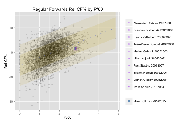
Bubble charts: The main look and design of the bubble charts, with four variables displayed simultaneously, comes from Rob Vollman’s Player Usage Charts, including the starting variables: x-axis for zone starts, y-axis for quality of competition, color for Relative Corsi. Our expansions and additions include every variable we have at our disposal including different game and score states.

Hextally: Directly inspired by Kirk Goldsberry’s NBA Shot Charts for Grantland and 538 (but perhaps the lack of a player with an appropriate name in the NBA made it difficult.) Expanded for both shot success probabilities (standard for basketball) and the rate of shots taken from each area of the ice (not standard for basketball, even if it were played on the ice.)

Shift Charts: We started with the original NHL shift charts before adding our own features. Both ShiftChart.com and timeonice.com (now defunct) hosted their own versions, inspiredby the same NHL.com template.

Shot Attempt Timelines: ExtraSkater (defunct) made them popular, but Behind The Net had the first ones we could find online.

Pulling the Goalie: Original post is here.

Raw Teammate/Competition Statistics:

For each of the teammate and competition statistics, relative numbers on a game by game basis by taking an exponentially weighted prediction of the next game’s numbers.

• TOIT60, TOIC60: The average time on ice per 60 minutes for teammates and competition in previous games, weighted by mutual time on ice.
• CorT%, CorC%: The share of Corsi events for the teammates and competition in previous games, weighted by mutual time on ice.
• tCF60, cCF60: The rate of Corsi events recorded on-ice for the teammates and competition in previous games, weighted by mutual time on ice.
• tCA60, cCA60: The rate of Corsi events recorded on-ice against the teammates and competition in previous games, weighted by mutual time on ice.

Other:

• Penalties: PN are non-coincidental penalties taken by a player; PN- are non-coincidental penalties drawn by a player. PenD is the difference, PN- minus PN; PenD60 is the net rate of penalties drawn every 60 minutes.
• Faceoffs: FO_W are faceoff wins. FO_L are faceoff losses. FO%^ is a shrunken faceoff win percentage, to avoid extreme results: identical to FO% if more than 20 faceoffs were taken, a combination of this and a 40% success ratio if less.
• Zone starts: ZSO, ZSN and ZSD are the number of faceoffs taken in the offensive, neutral and defensive zones for which the player was present; ZSOoff, ZSNoff and ZSDoff are the number of faceoffs taken in the offensive, neutral and defensive zones for which the player was absent. ZSO% is the share of offensive starts divided by the offensive plus defensive. ZSO%Off is the share of offensive starts for when that player is absent; ZSO%Rel is ZSO% minus ZSO%Off.
• GV are giveaways, TK are takeaways. HIT are hits taken, HIT- are hits absorbed. None of these are recorded reliably in NHL buildings.

The WAR On Ice operation is looking for new people to help keep the site operations going. Can we count on you?

We have a few objectives with the site, moving forward:

1. Keep data accessible. We know that you like downloading things into a .csv and then doing magic with Excel, or R, or Python, or your abacus. We’re not going to change that. In fact, we’d like to make it easier for you to do.
2. Act as a community portal for new projects. Have you been working on a project, and you’d like it hosted somewhere? Particularly if it uses our data to start with, if it survives vetting, we’ll work with you and help to get it online.
3. Maintain accurate information. We want to uphold our reputation as a reliable source of data first and foremost.
4. Solve the “bus problem”. That is: if one of us gets hit by a bus, the site should keep on going.

You should join up if you want to give back to the community that you enjoy so much, by honing your own data-ninja skills on stuff that you know will help people out.

You shouldn’t join up if:

1. You want to make any money off this enterprise. Our ad revenue and donations feed straight back into server costs. If there’s anything left over, we donate back to the community or to charities recognized by the community.
2. You want to become super famous. Your time would probably be better spent making YouTube videos or animated GIFs like others we love.
3. You enjoy the blissful ignorance of how the data gets created in the first place and what could be wrong with it.

If you’re still interested, here are some more details about the site.

We tend to divide site operations into two categories:

1. Database Creation: Our database is assembled by starting with a number of different sources: for in-game information, NHL.com and sportsnet.ca; for roster info, NHL.com and TSN; for contract and transaction data, we’ve curated our own sources. Getting this data into a usable format is no easy task, let alone integrating it all into a common framework. This is going to be even more work when the NHL decides to completely overhaul their data back-end, which we expect to happen sometime mid-season with no advance notice. Responsibilities to be taken on:
   • Scraper/Manipulator Extraordinaire: Maintain the creation of our master database from original game sources.
   • Contract/Cap Guru:  Maintain and possibly add to our original database of contracts.
   • Database Manager: Take the previous two parts and integrate them together in the back end so anyone else in the community can use them with ease.
   • Quality Control: When someone does something new, run validations to make sure nothing else went to hell.
2. App Creation: What good is data if we have no way to show it? Right now, we have a variety of “apps” running on WAR On Ice that allow users to query information and see it displayed in semi-aesthetically pleasing tables and charts. Yes, we know that they’re slow. That’s where you come in. You can write applications that will hook into our data — skater performance, contract information, whatever your heart desires. Right now, most of our apps are built in Shiny, but for longer-term solutions, they need to be translated into something more efficient and less server-intensive. (Servers are expensive). If everything is built upon a common database format, anyone can develop their own apps on top of this without necessarily relying on our coding method. Responsibilities to be taken on:
   • Existing apps: Take the old app structure from Shiny and rebuild them as you see fit from our back-end.
   • New apps: Build you own apps, extending the ones we already have. This may include working from your own ideas or ideas from the community.
   • Graphics Specialist: Design new interactive graphics for our current modes that are even spiffier, and shareable/exportable to a wider audience.

Still with us? If you are interested in joining the team, please send us a note to waronice.com@gmail.com. Please include: the responsibilities you’re interested in and any prior experience you have.

We announced yesterday on Twitter that we’ve been working to rebuild the capacities of CapGeek from the ground up. Our biggest issue is taking raw contract information from a primary source and turning that into the database for use. Our second-biggest issue is making sure that we don’t take this data from any other public site — especially CapGeek’s archived pages. (We have no problem transforming existing public sources of data, but this salary info is the direct result of someone else’s hard work, not a value-added derivative.)

We got an extremely healthy response to our original query for help in doing this cross-checking of data. Once we’ve made some progress on this, we’ll open up the database for a public examination; following this, we plan to have some more of the tools built and available for use well before the trade deadline.

The only other issue is what to call it: RecapGeek is a fine name for the rebuilding project but not the services, and war-on-ice-cap sounds like we’re either pro-global-flooding or anti-Tim-Horton’s.

We’ve recently been integrating a lot of new data into the site, with more to come. But we have some major changes to announce as things move forward.

1) The big one: we now have x,y data for all shot attempts going back to the 2005-2006 season as obtained from the ESPN feed. We note that since a fraction of games didn’t have GameCast information, we had to stitch it together a bit by imputing locations, taken by matching the distance of the unknown shot to another taken by the same player of the same type. This got particularly interesting when looking at buildings that didn’t seem to have any tracking within a season — Montreal in 2006-2007 — but it’s as good as we’re going to get right now, and far better than we had before.

This means that we’ve immediately extended Hextally back to 2005-2006, and augmented it with all shot attempts, blocked and unblocked. (Goalie Hextally just has saves and goals as before.) You’ll see some more features with this data being rolled out soon.

2) We made a tweak to our three “danger zones“, including facetiously naming them as such. (UPDATE, 2014-12-10: Apparently a similar name has been in use for years in soccer, so we can’t even take real credit for an idea that filtered through to us via Fangda Li.) The high slot range now reaches above the home plate line, and the “center point” is now considered low danger. Here’s one such map with numbers for the Kings this season:

This lines up better with goal probabilities in each zone.

3) We’ve simplified our rink adjustment factor to operate on distance. For each rink in consideration, we compare the cumulative distribution functions (CDFs) of shots for that team at home vs. that team away, in two groups only (slap shots and non-slap shots), and change the distance of a shot in a building to match its position on the other CDF. So if a shot was at the median distance of 25 feet at Madison Square Garden, and the median for all shots involving the Rangers away was 28 feet, the distance would be so adjusted. The (x,y) coordinate is changed by maintaining the angle from the center of the net and stretching out or shrinking in.

This is a precursor to a better system to be deployed at a future date, but for most of our purposes, it’s distance deflation that causes problems in these models, and as you can see from the danger zone chart, distance is roughly concordant with zone.

4) We got rid of “close” measurements. There were reasons for this:

• It’s less predictive of future behaviour than unadjusted but full data. Particularly the drag on scoring in tied games near the end of regulation.
• We’re going to be adding score-adjusted measures soon, which are better for that.

All in all, there’s more on the horizon that we’re committing to. Stay tuned.

 

We’ve made a few big changes to the site in the last little while that we’re testing out right now. Recent upgrades include:

• An overhaul of Hextally for teams and players, to better interface with the rest of the site.
• A brand-new Hextally for goaltenders focusing on shooting percentages by zone. It serves mainly to show how statistically insignificant the differences from average are for any goalie.
• New labs entries: Bench assists and Gordie Howe hat tricks, because they’re fun to read.

More is coming soon as we integrate new data sources.

We’re gratified by all the people who a) ask how they can help us out, and/or b) tell us what’s wrong with the site. This is intended to be a community resource, so the more constructive feedback we get, the better.

A few things you can do:

1) You have a suggestion for something you’d like on the site, especially something that needs a detailed description: please email us at waronice.com@gmail.com and let us know. We’re fairly responsive on Twitter but the plus-140 detail of email will help a lot.

2) Something is broken on the site: email or tweet to us.the more detail you can provide, the quicker we can get to it.

3) You like the site and want to share it: please mention us on Twitter, either the site @war_on_ice or either of us personally at @acthomasca and @stat_sam.

4) You used our tables or charts in a post or an analysis, or there’s something specific you’d like to share: please link to the page using the link we provide at the bottom.

5) You want to make a donation to help support our server costs or our workshop expenses: click the Donate button on the main page at war-on-ice.com! We promise that it’ll be applied only to support the site’s operations, not as payment for us to make the site — this is work our own time.

6) You want custom analyses not to be shared with others: contact us directly.

Who We Are

We are Andrew C. Thomas (@acthomasca) and Samuel L. Ventura (@stat_sam), statisticians by training, at Carnegie Mellon University in Pittsburgh.

Andrew was born in Toronto; Sam in Pittsburgh. While we are both fans of our respective home teams, WAR On Ice is a strictly non-partisan site and resource.

We watch the games.