Author Archives: @stat_sam

GUEST POST: Hockey and Euclid — Introduction to Bombay Ratings

Note:  This is part two of a series of guest posts written by @MannyElk.  In the first installment of Hockey and Euclid, Manny outlined the player similarity calculation used in the Similarity Calculator. The explanations to follow will assume knowledge from that article, so we urge anybody who wishes to understand the derivation of the Bombay function in detail to get caught up.  

We at www.war-on-ice.com are happy to host Manny’s newest Bombay Ratings App!  We continue to encourage others in the hockey research community to follow Manny’s lead and develop public applications that will further the frontiers of research in hockey analytics.

While working on the Similarity Calculator, I stumbled upon a study in which Euclidean distance was used to compare NBA players to Michael Jordan.  The author used the distances to generate a list of the most similar players to the man most would agree is the best ever.  From this idea, Bombay ratings were just a conceptual hop, skip and jump away.  Instead of choosing my own Michael Jordan from a list of historical players, I invented one.

Continue reading

GUEST POST: Hockey And Euclid — Calculating Statistical Similarity Between Players

Editor’s note:  This is a guest post written by Emmanuel Perry.  Manny recently created a Shiny app for calculating statistical similarities between NHL players using data from www.war-on-ice.com.  The app can be found here.  You can reach out to Manny on Twitter, @MannyElk.

We encourage others interested in the analysis of hockey data to follow Manny’s lead and create interesting apps for www.war-on-ice.com.

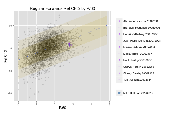
The wheels of this project were set in motion when I began toying around with a number of methods for visualizing hockey players’ stats.  One idea that made the cut involved plotting all regular skaters since the 2005-2006 season and separating forwards and defensemen by two measures (typically Rel CF% and P/60 at 5v5).  I could then show the position of a particular skater on the graph, and more interestingly, generate a list of the skaters closest to that position.  These would be the player’s closest statistical comparables according to the two dimensions chosen.  Here’s an example of what that looked like:
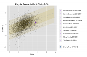
mh_s (1)

(click to enlarge)

The method I used to identify the points closest to a given player’s position was simply to take the shortest distances as calculated by the Pythagorean theorem.  This method worked fine for two variables, but the real fun begins when you expand to four or more.

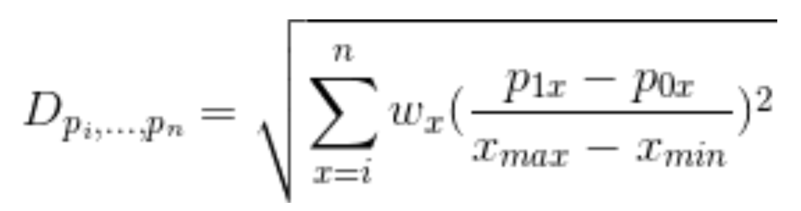
In order to generalize the player similarity calculation for n-dimensional space, we need to work in the Euclidean realm.  Euclidean space is an abstraction of the physical space we’re familiar with, and is defined by a set of rules.  Abiding by these rules can allow us to derive a function for “distance,” which is analogous to the one used above.  In simple terms, we’re calculating the distance between two points in imaginary space, where the n dimensions are given by the measures by which we’ve chosen to compare players.  With help from @xtos__ and @IneffectiveMath, I came up with the following distance function:

distance

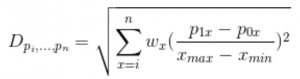
And Similarity calculation:

similarity

In decimal form, Similarity is the distance between the two points in Euclidean n-space divided by the maximum allowable distance for that function, subtracted from one.  The expression in the denominator of the Similarity formula is derived from assuming the distance between both points is equal to the difference between the maximum and minimum recorded values for each measure used.  The nature of the Similarity equation means that a 98% similarity between players indicates the “distance” between them is 2% of what the maximum allowable distance is.

To understand how large the maximum distance is, imagine two hypothetical player-seasons.  The highest recorded values since 2005 for each measure used belong to the first player-season; the lowest recorded values all belong to the second.  The distance between these two players is the maximum allowable distance.

Stylistic similarities between players are not directly taken into account, but can be implicit in the players’ statistics.  Contextual factors such as strength of team/teammates and other usage indicators can be included in the similarity calculation, but are given zero weight in the default calculation.  In addition, the role played by luck is ignored.

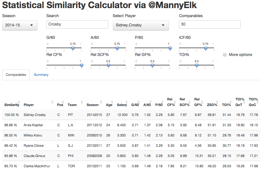
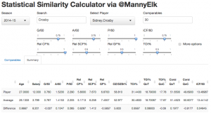
The Statistical Similarity Calculator uses this calculation to return a list of the closest comparables to a given player-season, given some weights assigned to a set of statistical measures.  It should be noted that the app will never return a player-season belonging to the chosen player, except of course the top row for comparison’s sake.
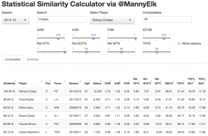
app-comparables

(click to enlarge)

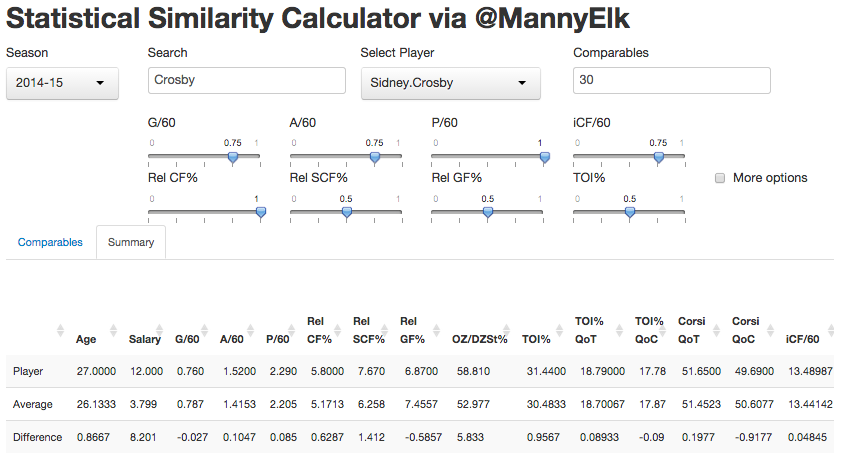
Under “Summary,” you will find a second table displaying the chosen player’s stats, the average stats for the n closest comparables, and the difference between them.

app-summary

(click to enlarge)

This tool can be used to compare the deployment and usage between players who achieved similar production, or the difference between a player’s possession stats and those of others who played in similar situations.  You may also find use in evaluating the average salary earned by players who statistically resemble another.  I’ll continue to look for new ways to use this tool, and I hope you will as well.

** Many thanks to Andrew, Sam, and Alexandra of WAR On Ice for their help, their data, and their willingness to host the app on their site. **

Sam’s Zone Transition Time Paper

In November, I introduced a preliminary version of my work on “Zone Transition Times” (ZTTs) at the Pittsburgh Hockey Analytics Workshop.  The slides for and video of my presentation can be found here.

In December, I submitted a paper on ZTTs to the Sloan Sports Analytics Conference; the paper was not selected as a finalist in the research paper competition.  A slightly modified version of this paper can be found here.  The results and text are unchanged from the December submission, except for minor typos.

Since then, I’ve identified some flaws with this work that I didn’t (have time to) explore in November/December:

Continue reading

NHL Salary Cap FAQ — Mike Colligan

Our running list of Frequently Asked Questions on the NHL Salary Cap, provided by site partner Mike Colligan.

For more from Mike Colligan, visit Colligan Hockey.

[WAR Off Ice] Updates to Bergeron and M. Staal Contract Info

Over the next few weeks, we will be releasing salary cap charts and information for NHL teams under the unofficial name, “WAR Off Ice”.  Leading up to the full release, we’ll post important contract news to the WAR On Ice blog.

We’re pleased to release early information on two player contracts today.  First, the widely reported contract terms for Patrice Bergeron are incorrect, according to two verified, high level sources.  Additionally, we have what were (to our knowledge) previously unreleased details on the structure of Marc Staal’s contract.

In Bergeron’s case, the average annual value (AAV) of his contract ($6.875M) is higher than what has been publicly reported to-date ($6.5M).  Staal’s AAV is $5.7M, same as previously reported.

Bergeron

Before today, it was publicly believed that Bergeron and the Bruins agreed to an 8 year, $52M contract ($6.5M AAV).  However, our sources have confirmed that they actually agreed to an 8 year, $55M contract ($6.875M AAV), structured as follows:

  • Years 1-4:  $8.750M salary, $0.0M bonus
  • Year 5:  $0.875M salary, $6.0M bonus
  • Year 6:  $0.875M salary, $3.5M bonus
  • Years 7-8:  $3.375M salary, $1.0M bonus

Bergeron will be 36 years old when the contract expires after the 2021-22 season.  We do not know at this time what implications this has for the Bruins’ salary cap situation for the 2014-15 season.

Staal

Below are details on the structure of Marc Staal’s contract with the Rangers, which goes into effect next season and expires after the 2020-21 season: UPDATE: this was reversed originally. Below is now correct.

  • Year 1 (2015-16):  $4.0M salary, $3.0M bonus  — $7.0 M total
  • Years 2-4 (2016-17 — 2018-19):  $5.0M salary, $1.0M bonus — $6.0 M total/y
  • Year 5 (2019-20):  $4.0M salary, $1.0M bonus — $5.0 M total
  • Year 6 (2020-21):  $4.0M salary, $3.0M bonus — $4.2 M total

Again, this results in a $5.7M AAV for the Rangers.

All of this information will be available soon on our NHL team salary cap charts site.

Predictability Differences for Forwards and Defensemen

Note:  If you haven’t yet read our post on how SCF% better predicts future GF% than does CF%, we recommend reading that first.  The definitions of metrics, data used, and methodology used in this post is the same as what is written here, so we refer interested readers to there for more info.

Summary:  This is an update to our previous post on the best metrics for predicting player performance.  Here, we split the analysis out by position (forwards vs. defensemen).

In this analysis, using all data going back to the 2005-06 NHL season:

  1. For forwards, SCF% is the best predictor of future GF% of the metrics we tested
  2. For forwards, CF% is a better predictor of future GF% than is FF%, but for defensemen, the opposite is true.
  3. For defensemen, FF% is the best predictor of future GF% (with SCF% finishing a close second) of the metrics we tested.
  4. SCF% is a much better predictor of future GF% for forwards than it is for defensemen.
  5. In general, future GF% is more accurately predicted for forwards than it is for defensemen.

Continue reading

Better Than Corsi: Scoring Chances More Accurately Predict Future Goals For Players

Summary:

Since the 2005-06 NHL season, the percentage of Scoring Chances For (SCF%) is a better predictor of future Goals For (GF%) than Corsi For (CF%) is for individual players.  (Under specific conditions, of course, but it’s promising either way.)

Combining data across all seasons since 2005-06, the season-to-season correlations are:

  1. cor(Past SCF%, Future GF%) = 0.322
  2. cor(Past CF%, Future GF%) = 0.311
  3. cor(Past GF%, Future GF%) = 0.287

Using multiple linear regression and combining across all seasons, we find that:

  • For every one-percentage-point increase in SCF%, future GF% is expected to rise by about 0.41 percentage points, holding all other variables constant.
  • For every one-percentage-point increase in CF%, future GF% is expected to rise by about 0.22 percentage points, holding all other variables constant.

Continue reading

Density Plots for Modern Hockey Statistics (Warning: There’s Math, But It’s Useful Math)

At #PGHAnalytics on Saturday, there was a short discussion about uncertainty in metrics such as Corsi% and Fenwick%.  How can we quantify this uncertainty / variability?  The simplest way to do this would be to include standard errors with each player rating such as Corsi% or Fenwick%, which is a good start.  What else can we do?

Suppose we told you that you could choose between two hypothetical players, and the only pieces of information we gave you about them were their respective 5-on-5 Close Corsi%s from the first 10 games of the season:

Player A:  90%, 70%, 30%, 33%, 50%, 75%, 25%, 80%, 90%, 22%

Player B:  55%, 60%, 44%, 55%, 58%, 63%, 55%, 66%, 45%, 66%

Which would you choose?  Why?

After the jump, we introduce a graphical approach to comparing pairs of players, looking at the distribution of their single-game Corsi%s, Fenwick%s, and much more.

Continue reading