At #PGHAnalytics on Saturday, there was a short discussion about uncertainty in metrics such as Corsi% and Fenwick%. How can we quantify this uncertainty / variability? The simplest way to do this would be to include standard errors with each player rating such as Corsi% or Fenwick%, which is a good start. What else can we do?
Suppose we told you that you could choose between two hypothetical players, and the only pieces of information we gave you about them were their respective 5-on-5 Close Corsi%s from the first 10 games of the season:
Player A: 90%, 70%, 30%, 33%, 50%, 75%, 25%, 80%, 90%, 22%
Player B: 55%, 60%, 44%, 55%, 58%, 63%, 55%, 66%, 45%, 66%
Which would you choose? Why?
After the jump, we introduce a graphical approach to comparing pairs of players, looking at the distribution of their single-game Corsi%s, Fenwick%s, and much more.
Player A is the more up-and-down player, turning in some great performances and some poor ones. Player B is the more consistent player, turning in performances that are usually above-average, and at worst very close to average. (Both players are fictitious, but similar types can easily exist.)
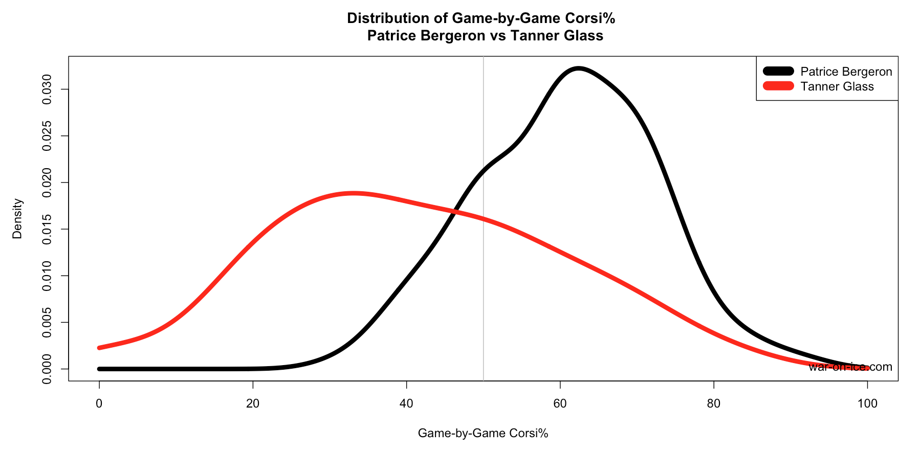
We’re not going to tell you which player you should prefer, since there are clearly pros and cons to both. Instead, we provide a tool to help you compare players: a smoothed density plot of game-by-game outcomes to give a sense of what you can expect from them in future games. For example, we can show that Patrice Bergeron is highly likely to give a better 5-on-5 Corsi% than Tanner Glass:
What The Heck Is A Density Plot?
For those who haven’t seen these before, a density plot is essentially a histogram shown at a continuous scale: It shows the distribution of values that a given variable (e.g. Corsi%) takes, along with how likely/common each particular value is.
The x-axis shows the range of possible values of the given variable (in the above graph, Corsi% at 5-on-5 since 10/1/2013). The y-axis shows the “density” of the distribution of observed values of that variable. Higher densities (y-axis) mean that the corresponding value of the given variable (x-axis) is more likely; lower densities mean that the corresponding value of the given variable is less likely.
In the above plot, Patrice Bergeron’s Corsi% distribution (black curve) has a large mode around 60% (in other words, really good), meaning it’s common for him to have Corsi%s around 60% in a single game. Bergeron’s density curve drops off around 40% and 80%, meaning it’s fairly uncommon for him to have Corsi%s below 40% or above 80%.
Tanner Glass’s Corsi% distribution (red curve) has a mode around 35% (in other words, really bad). His distribution is much wider, indicating that his Corsi% is much more variable than Bergeron’s. As @senstats pointed out on Twitter, this is likely because Glass typically has a low 5-on-5 TOI in any particular game, which will make these numbers more variable, so we have to note these things when picking our comparable players.
OK, But What Does The Density Curve Actually Mean, and How Did You Get It?
The curve represents what’s called a “kernel density estimate“. We use it to estimate what the data would look like if we had much more of it available, but also — and most importantly for our purposes here — to smooth out the data to make it easier to visualize. A histogram does the same thing — it smoothes data by counting it in blocks/bins — but it can be harder to compare two of those at once, and nearly impossible to compare three or more.
A player’s density curve for a given statistic shows an estimate of the probability density function for that player/stat. The main use of this is to estimate a probability that something will happen in a future game if little changes. For example, the probability that Patrice Bergeron will have a Corsi% greater than 50 is the total area under the curve where that’s the case:
P(Bergeron’s Single-Game Corsi% > 50) = [area under Bergeron's curve where the x-axis > 50]
Some additional details:
- See R’s help file for the density function for more information.
- In the above link, go to “Details” for more on kernel density estimation.
- We fix the density to be between 0 and 100 for percentages like Corsi% and Fenwick%.
- Otherwise, we used the default settings for all players/stats.
- We intended for these to be used for continuously valued stats only (e.g. Corsi%, OnIceSh%, etc), but we’ll update this later on with similar plots for discrete-valued stats (e.g. # of shots, +/-), since the primary purpose is to make the full distribution of data easier to see, rather than being able to reassemble the raw data.
In the statistical programming language R, which we used to build WAR On Ice, we used the density function to calculate the kernel density estimate for each player/stat.
How Can I Make My Own Density Plots?
On war-on-ice.com, you can create these graphs for yourself for any variable, any situation, and any pair of players:
- Under the Players drop-down menu, select Skater History and click the By Game tab.
- Select your home/away situation, score situation, man-strength situation, etc.
- Enter the first player’s name in the “Filter Player” textbox at the top of the page.
- Scroll down below the table and enter the second player’s name in the “Filter Players” textbox.
- Choose which variable you want to use to compare your players.
Two graphs should show up: First, the moving average graph of the chosen variable over time for both players. Second, the density plot comparing the distribution of the chosen variable for both players.
Additional Examples
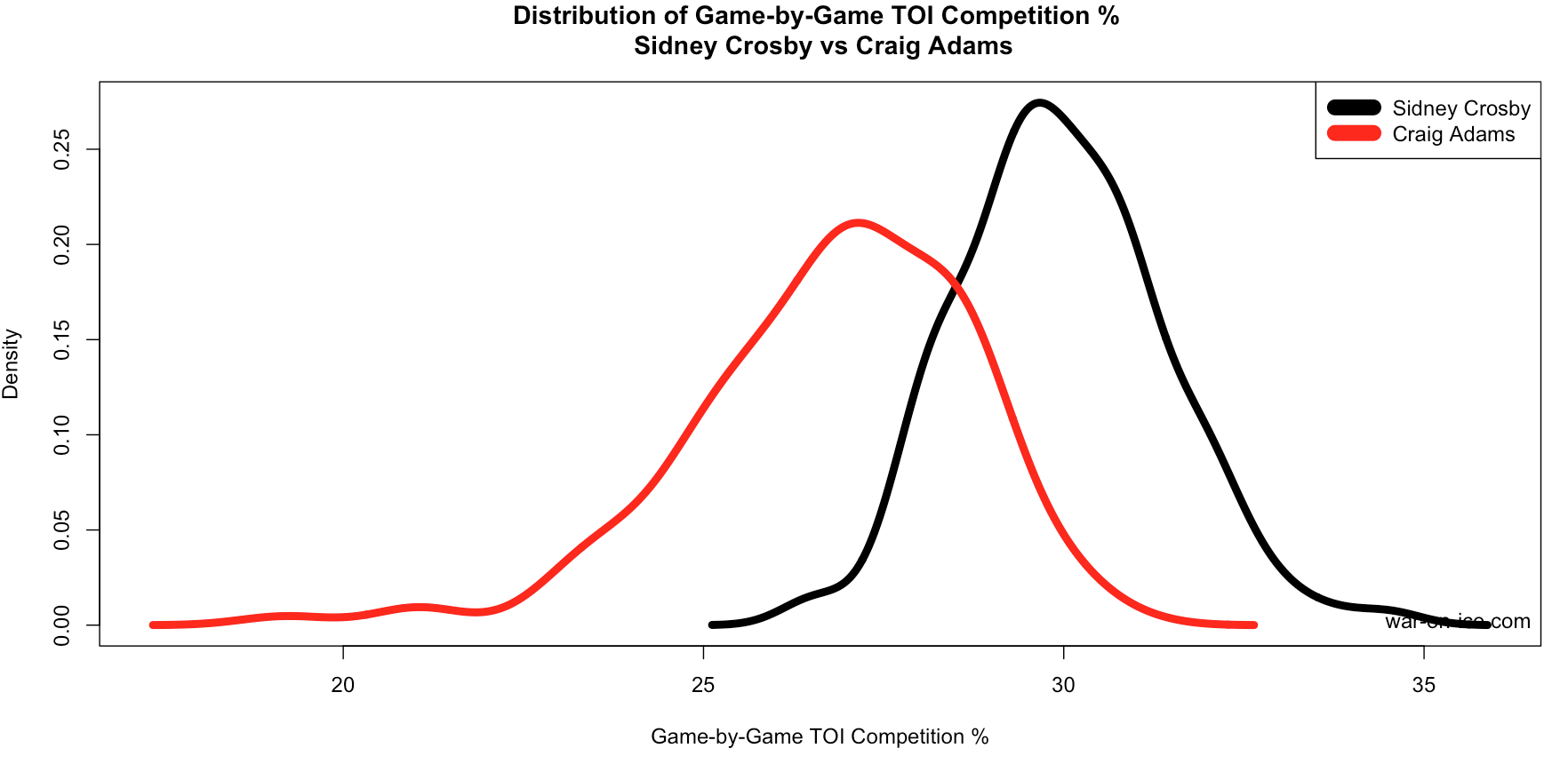
Above: QoC-TOI since 10/1/2013 at 5-on-5 for Sidney Crosby and Craig Adams. As expected, Crosby consistently faces much tougher competition, since there isn’t much overlap in these two distributions.
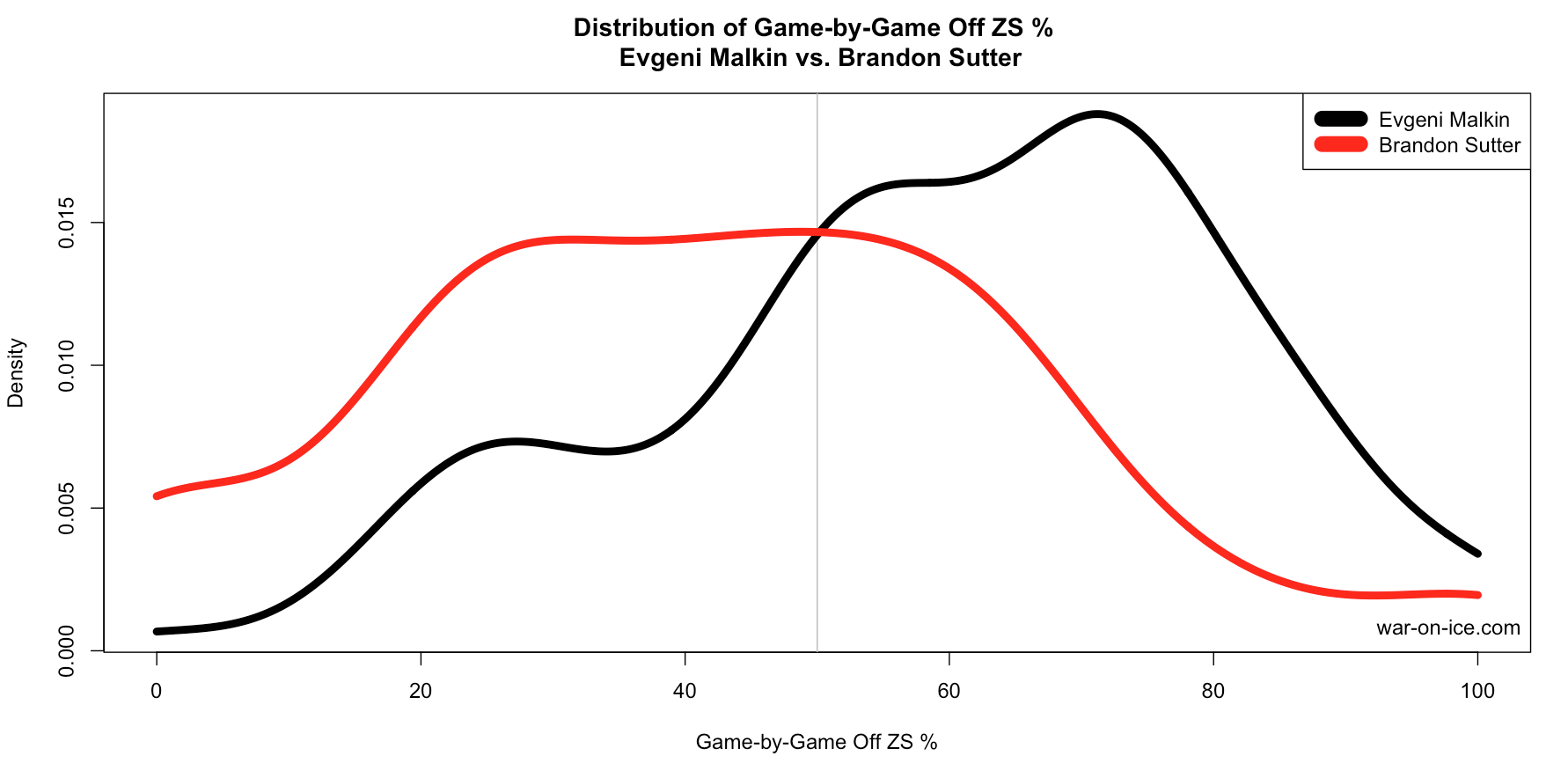
Above: Offensive Zone Start% since 10/1/2013 at 5-on-5 for Evgeni Malkin vs. Brandon Sutter. Dan Bylsma typically used Malkin heavily in the offensive zone, as evidenced by the mode in his density estimate around 70%. Brandon Sutter is typically used in a more defensive role, since a large mass of his distribution is below 50%.
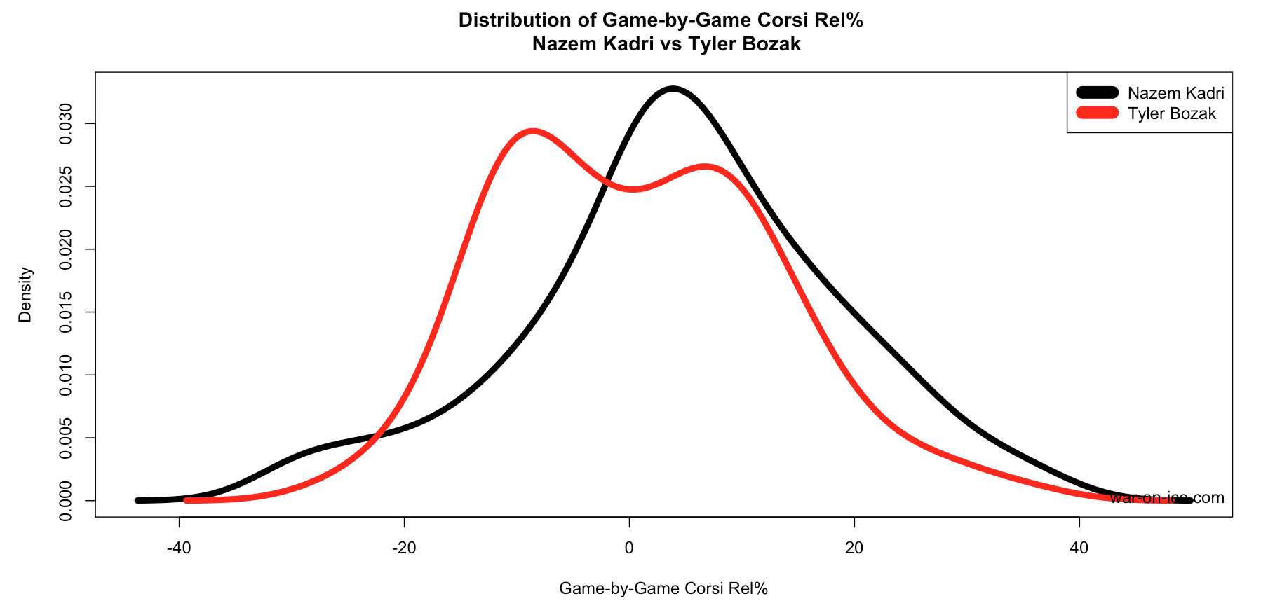
Above: Finally, the above graph shows Kadri vs. Bozak in Corsi% Rel at 5-on-5 since 10/1/2013. What’s interesting here is Bozak’s seemingly bi-modal distribution. One mode is above zero, and one mode is below zero, indicating that he has some good games, some bad games. Another interpretation of this is that sometimes he is used in more defensive roles, and sometimes in more offensive roles (since usage can impact Corsi% Rel).
Make some player comparisons with density plots of your own, and let us know what you think!
Pingback: Peyton Manning and the postseason | StatsbyLopez